 |
|
![]()
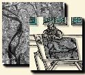
| Figure 17: Original
image
|
Figure 18: Fuzzy
radiometry
|
| Figure 19: MDRO
|
Figure 20: Conjunctive
fusion
|
Images (17 to 20) show a simple example of fusion on a SPOT P image, using two operators, one for the radiometry (it codes how the radiometry of a pixel is similar to the radiometry of a dried river) and the MDRO.
The result of the DUDA operator (Figure 19) is very noisy. The combination using simple conjunctive fusion (Figure 20) gives a best result and the line is thinner.
The dynamic programming is then performed on image (Figure 17). A segment from a hypothetical database (Figure 21) is used to determine a search area ( Figure 22) (for the example a single straight line, placed manually).
Left side of the area is the source set of points and the right side is the target one.
A modification of the original algorithm allows selecting and fixing one best initial point in the source set. Without this constraint the path starts approximately at the center of the left side of image ( Figure 22) and we cannot detect the path which is in the upper left corner.
| Figure 21: Original
segment
|
Figure 22: Search
area
|
| Figure 23: Dynamic
algorithm
|
Figure 24: Blur
|
On the result shown on image ( Figure 23), can be seen an erratic path on the left part of image and mainly a horizontal S-like shape at the bottom and a straight line at the bottom of the hairpin bend. To correct these problems we use the snake-like algorithm.
As the algorithm tends to reach the summits of potential, we perform a linear blur ( Figure 24) on the fusion map to have more convex cross sections.
It is possible to tune two parameters, stiffness and control point separation. The stiffness controls the smoothing rate of the curve and the separation of points controls the level of detail.
Influences of the two parameters can be seen on figures 25 to 28:
| Figure 25: Flexible,
many points
|
Figure 26: Stiff,
many points
|
| Figure 27: Flexible,
few points
|
Figure 28: Stiff,
few points
|