 |
 |
![]()
![]()
Let us reconsider the problem, posed in the previous pages, of designing a classifier to separate two kinds of marble pieces, Carrara marble and Thassos marble.
Suppose that an observer, watching marble emerge from the mill, finds it so hard to predict what type will emerge next, that the sequence of types of marble appears to be random.
Using decision-theoretic terminology, we say that as each piece of marble
emerges, nature is in one or the other of the two possible states: either
the marble is Carrara marble, or Thassos
marble. We let ![]() denote the state of nature, with:
denote the state of nature, with:
Because the state of nature is so unpredictable, we consider ![]() to be a random variable.
to be a random variable.
If the mill produced as much Carrara marble than Thassos marble, we
would say that the next piece of marble is equally likely to be Carrara
marble or Thassos marble. More generally, we assume that there is some
a priori probability P(![]() )
that the next piece is Carrara marble, and some a
priori probability P(
)
that the next piece is Carrara marble, and some a
priori probability P(![]() )
that the next piece is Thassos marble. These a priori probabilities reflect
our prior knowledge of how likely we are to see Carrara marble or Thassos
marble before the marble actually appears. P(
)
that the next piece is Thassos marble. These a priori probabilities reflect
our prior knowledge of how likely we are to see Carrara marble or Thassos
marble before the marble actually appears. P(![]() )
and P(
)
and P(![]() )
are non negative and sum to one.
)
are non negative and sum to one.
Now, if we have to make a decision about the type of marble that will appear next, without being allowed to see it, the only information we are allowed to use is the value of the a priori probabilities. It seems reasonable to use the following decision rule:
![]()
In this situation, we always make the same decision, even though we know that both types of marble will appear. How well it works depends upon the values of the a priori probabilities:
In general, the probability of error is the smaller of ![]() and
and ![]() .
.
In most circumstances, we have not to make decisions with so little evidence. In our example example, we can use the brightness measurement x as evidence, as Thassos marble is lighter than Carrara marble. Different samples of marble will yield different brightness readings, and it is natural to express this variability in probabilistic terms; we consider x as a continuous random variable whose distribution depends on the state of nature.
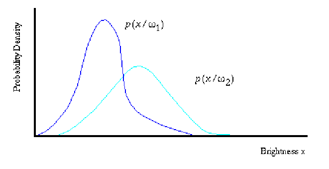
Let ![]() be the state-conditional probability density
function for x, i.e. the probability density function for x
given that the state of nature is
be the state-conditional probability density
function for x, i.e. the probability density function for x
given that the state of nature is ![]() .
Then, the difference between
.
Then, the difference between ![]() and
and ![]() describes the difference in brightness between Carrara and Thassos marble
(see figure 16)
describes the difference in brightness between Carrara and Thassos marble
(see figure 16)
 |
Suppose that we know both the a priori probabilities ![]() and the conditional densities
and the conditional densities ![]() .
Suppose further that we measure the brightness of a piece of marble and
discover the value of x. How does this measurement influence our
attitude concerning the true state of nature? The answer to this question
is provided by Bayes' rule:
.
Suppose further that we measure the brightness of a piece of marble and
discover the value of x. How does this measurement influence our
attitude concerning the true state of nature? The answer to this question
is provided by Bayes' rule:
|
(3) |
where
|
(4) |
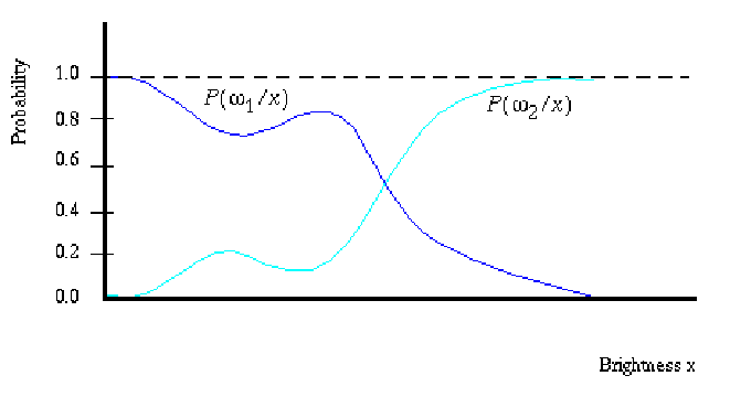
Bayes'rule shows how the observation of value x changes the a
priori probability ![]() into the a posteriori probability
into the a posteriori probability
![]() .
Variation of
.
Variation of ![]() with x is illustrated in Figure 17
for the case
with x is illustrated in Figure 17
for the case ![]() and
and ![]() .
.
 |
If we have an observation x for which ![]() is greater than
is greater than ![]() ,
we would be naturally inclined to decide that the true state of nature
is
,
we would be naturally inclined to decide that the true state of nature
is ![]() .
Similarly, if
.
Similarly, if ![]() is greater than
is greater than ![]() ,
we would be naturally inclined to choose
,
we would be naturally inclined to choose ![]() .
.
To justify this procedure, let us calculate the probability of error whenever we make a decision. Whenever we observe a particular x,

Clearly, in every instance in which we observe the same value for x, we can minimize the probability error by deciding:
Of course, we may never observe exactly the same value of x twice.
Will this rule minimize the average probability of error? Yes, because
the average probability of error is given by:

and if for every x, P(error/ x) is as small as possible, the integral must be as small as possible. Thus, we have justified the following Bayes' decision rule for minimizing the probability of error:
This form of the decision rule emphasizes the role of the a posteriori probabilities. By using equation 3, we can express the rule in terms of conditional and a priori probabilities.
Note that p(x) in equation 3
is unimportant as far as making a decision is concerned. It is basically
just a scale factor that assures us that ![]() .
By eliminating this scale factor, we obtain the following completely equivalent
decision rule:
.
By eliminating this scale factor, we obtain the following completely equivalent
decision rule:
Some additional insight can be obtained by considering a few special cases:
In general, both of these factors are important in making a decision, and the Bayes' decision rule combines them to achieve the minimum probability of error.