The final resulting regions are used to determine the samples of the two classes (built up/non-built up areas) on the previous computed similarity image (Figure 63). Both built up and non-built up classes are supposed to appear in the image. This algorithm is made of two steps:

• The first step is the choice of a first threshold value on the image, in order to separate the pixels in two classes. This threshold is chosen in order to obtain at least one region with more than 60 percent of built up pixels and another one with more than 60 percent of non-built up pixels. The method is based on dichotomy. A first threshold value is fixed. Then, the percentage of built up and non-built up pixels is computed for each region. If none of the regions contains more than 60 percent of built up pixels, the threshold value is reduced. In the same way, if none of the regions contains more than 60 percent of non-built up pixels, the threshold value is increased.
  
  
• The second step is the computation of a new threshold according to the previous one. A built up sample, corresponding to the region that contains the highest built up pixels percentage, and a non-built up sample corresponding to the region that contains the highest non-built up pixels percentage are chosen. The new threshold is computed by means of the normalized and filtered (with the 1D ISEF filter) histograms of the samples. The advantage of this filter is to preserve the localization of the extrema.




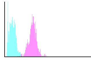
Starting Histogram



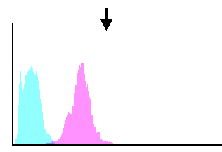
Filtered Histogram

The new threshold value is the intersection between the two filtered histograms' curves:

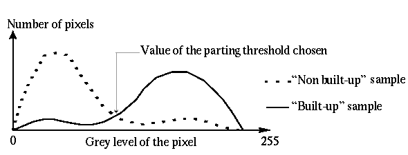
The algorithm ends when the new threshold value has already been computed.

This algorithm is insensitive to wrong segmentation as it only takes into account the best classified regions and it uses filtered histograms to compute the threshold value. If a sample contains some pixels of the other class, these pixels do not influence the choice of the new threshold. With the final samples (in about 4 to 5 iterations), a membership coefficient of a pixel to each of the two classes is defined by using the Bayes' rule.

First, the histograms are modified. For each grey level lower than the one that corresponds to the maximum of the histogram of the non-built up sample, the value of the histogram of the non-built up sample is equal to its maximum. In the same way, for each grey level upper than the one that corresponds to the maximum of the histogram of the built up sample, the value of the histogram of the built up sample is equal to its maximum.

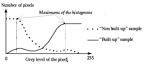
This transformation is made to eliminate the wrong classifications due to the deficiency of knowledge for some grey level values. The transformation can be applied because of the knowledge of the distribution of the two classes (based on the similarity measure of a pixel to a building). Then with these new ``histograms'', the membership coefficient of a pixel to the built up and non built up classes is defined:

h_u(g) is the value of the histogram of the built up area sample for the grey level g and h_nu(g) is the value of the histogram of the non built up area sample for the grey level g.