How to compute a histogram from samples of a class.

How to Compute a Histogram from Samples of a Class?

Figure 7 presents a zoom onto the two samples of class 3 in spectral band MSS4.

Tables 2 and 3 indicate the numerical values of grey levels taken by each pixel.

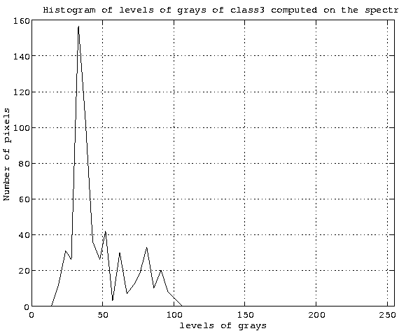
Table 4 presents the distribution of the pixels of the samples of class 3 in term of levels of grey. The histogram of grey levels for this class, in spectral band MSS4, is shown in figure 8.

It is noticed that this class is characterized mainly by grey levels 33 and 38, but also, with a less degree, by levels 62 and 81. We thus deal with classes which representative histograms have not purely a Gaussian shape.

**Table 2:** Grey levels of each pixel of the upper sample of class 3 in spectral band MSS4.
Higher sample
62	62	62	62	52	52	38	38	38	33	38	38	33	38	38	38	38
62	48	62	62	48	43	33	33	43	33	33	43	33	33	43	43	33
52	52	48	48	38	33	38	38	38	38	33	38	38	33	33	33	33
62	52	48	52	38	38	38	38	38	38	38	38	33	33	24	33	24
62	57	57	43	33	38	33	33	38	33	33	38	33	24	19	24	38
52	52	48	48	33	28	33	33	43	33	28	33	33	33	19	19	33
62	62	62	43	38	43	38	38	38	33	38	33	33	33	33	24	33
67	67	48	43	33	33	33	33	43	33	33	28	33	28	28	28	28
52	48	33	33	38	38	38	38	33	33	33	33	24	24	24	38	52
62	48	33	38	38	38	38	33	33	33	33	33	24	24	33	52	81
57	38	38	38	33	38	33	33	24	24	24	24	24	19	43	72	72
52	48	28	33	33	33	33	28	19	19	28	19	28	33	33	52	76
52	33	38	43	38	38	33	24	24	24	33	33	43	43	43	76	76
48	38	43	38	43	28	28	24	24	28	38	38	38	43	67	72	72
38	38	38	48	33	24	24	33	33	33	33	33	33	38	62	76	62
38	38	33	33	33	24	33	33	38	33	33	33	33	48	76	76	76
38	33	33	33	33	33	33	33	33	33	33	33	33	62	86	72	62

**Table 3:** Grey levels of each pixel of the lower sample of class 3 in spectral band MSS4.
Lower sample
38	38	38	33	33	33	19	24	52	91	91	91	81	62	48	48	48
38	38	38	33	33	33	24	24	48	81	81	81	81	76	52	52	62
38	38	38	38	43	24	19	33	52	67	86	91	91	101	86	67	62
33	43	43	33	33	28	19	19	33	28	48	81	86	81	86	81	67
38	38	38	33	33	33	38	38	33	52	81	96	96	96	81	81	72
43	33	28	33	33	33	33	33	43	62	81	101	91	91	91	91	72
38	33	33	33	38	24	33	38	48	52	81	91	91	81	81	76	62
33	38	38	38	38	33	33	48	52	48	81	96	81	81	81	76	76
38	33	33	38	33	33	43	52	43	52	91	101	91	101	91	91	72
28	28	19	28	33	28	28	43	43	43	52	76	86	81	86	76	76
33	33	33	38	33	33	33	43	52	52	52	76	96	81	96	81	72
28	33	33	28	33	28	33	43	62	62	72	81	81	91	81	81	72
24	24	33	38	33	33	48	52	52	76	81	62	52	76	76	91	91
33	38	33	38	38	48	52	48	62	81	62	52	38	52	81	96	91
33	38	38	38	43	52	52	62	43	43	38	24	62	91	86	86	67
33	33	33	33	33	48	52	52	43	33	33	28	33	52	81	86	81
38	38	33	38	52	62	52	43	38	38	38	38	52	52	72	81	96

**Table 4:** Distribution of the pixels by grey level for the samples of class 3 in spectral band MSS4.
Grey level	Number of pixels
19	12
24	31
28	26
33	157
38	103
43	36
48	26
52	42
57	3
62	30
67	7
72	12
76	18
81	33
86	10
91	20
96	8
101	4
Total	578

**Figure 8:** Histogram of the grey levels of class 3 for spectral band MSS4.
$\begin{figure}\epsfysize=10cm\epsfbox{c4-histo-classe3.eps}\end{figure}$

The training step consists in computing the histogram of grey levels of each class from its samples. This computation is carried out for each spectral band of the image and for each out-image data.

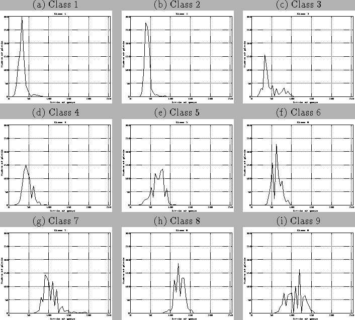
**Figure 9:** Histograms of each class for spectral band MSS4.
$\begin{figure}\begin{center}\par\begin{tabular}{ccc}(a) Class 1 & (b) Class 2......ize=3.9cm\epsfbox{c4-histo-p4-cl9.eps}\\\end{tabular}\end{center}\end{figure}$

Figure 9 presents the histograms of the nine classes for spectral band MSS4. We can notice that they overlap rather largely. Some histograms are spread out, of low amplitude, and are embedded among the other histograms.

As classification is only based on the histograms which describe the classes, classes will be not easily distinguished from each other during classification. In particular, classes 3 and 4, which have a poorly spread out histogram, are merged with classes 1 and 2, which histogram is very narrow.

The preference, from these histograms, will be clearly given to classes 1 or 2 rather than 3 or 4. Classes 3 and 4 thus will be very badly recognized. From additional data providing from other sources, information fusion will help raising the confusion between these four classes, and improving the recognition of classes 3 and 4.

It is also noticed that classes are divided roughly into two groups:

classes 1 to 6, whose histograms have rather low grey levels (from 0 to 100 approximately), and
classes 7 to 9, for which the histograms have higher grey levels (from 60 to 200).

This duality is also present for the other spectral bands, but with different ranges of grey levels.

Let us recall that:

classes 1 to 6 correspond to forest or savanna and their samples are in the most mountainous part of the image (on the slopes or the plateaux), and
classes 7 to 9 are those of cultures and thickets, and their samples are situated in the plains.

These differences in vegetation types can be found in the histograms.

IRIT-UPS