Page 42



Practical Details

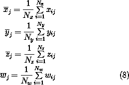
Let us say that we have 3 pure classes with spectral values in the j th band x_j, y_j and z_j respectively. Let us also assume that we have a mixed region with fractional cover a, b and 1-a-b from each pure class respectively. The spectral value of a mixed pixel in the jth band is w_j. From the sets of pure and mixed pixels we have, we can calculate the mean values of x_j, y_j, z_j and w_j, , , and respectively, as:

where N_x is the number of pixels that represent the first pure class, x_ij is the spectral value of the ith pixel in band j and the meaning of the remaining quantities is similar. It is known then that the following equation holds between , , and :

Next, we calculate the elements of the covariance matrix of each set of pixels, using the following formulae:

with similar formulae for C_yjk, C_zjk and C_wjk. In the above expression, C_xjk is the jk element of the covariance matrix of the x class. From the theory of random variables it is then known that the following relationship holds between the corresponding elements between the various covariance matrices:

It is possible to calculate 3rd moments for each distribution and make use of the relationships between them and derive another set of equations to be used alongside equations (9) and (11). Bosdogianni et.al. solved the set of equations (9) and (11) in the least square error sense. They chose values a and b so that the sum of the square of the errors with which equations (9) and (11) were satisfied was minimum. However, acknowledging the fact that the mean of a distribution is computed in a more reliable way than the covariance matrix, they weighted each error inversely proportionally to the standard error with which each statistic can be estimated. So, they chose a and b so that the following expression was minimised:




	What if we do not have data to represent the pure classes?
	Advantages of the approach
	Disadvantages of the approach
	Relationship with the simultaneous unmixing of sets of mixed pixels